Wind power is a variable energy source depending on local wind velocity changes. Having an accurate prediction of these wind changes improves grid integration and management. Here we offer the results of a high resolution implementation of the WRF-ARW model for the Iberian Peninsula and Canary Isles. Current model has a grid cell size of 9 km, which allows a better definition of local topography effect on wind. For complex topography it is possible to run the model at higher resolution, through nested domains at decreasing cell size, in order to achieve a more detailed simulation. Boundary and initial conditions are provided by the GFS 0p25 global model at 0.25° resolution.
GFS is the acronym of Global Forecast System, which is run four times a day by the US National Weather Service. The outputs are available at 2.5, 1, 0.5 and since January 2015 at 0.25 degrees of resolution.
The Weather Research and Forecasting (WRF) Model "is a next-generation mesoscale numerical weather prediction system designed to serve both atmospheric research and operational forecasting needs. It features two dynamical cores, a data assimilation system, and a software architecture facilitating parallel computation and system extensibility" [1]. The WRF is a collective effort by many scientists over the world and is regularly updated and upgraded.
On mountain regions the resolution of the model is important in order to simulate the impact of topography on weather systems. At 0.25° or 0.50° resolution, global models do not represent mountain ranges accurately, missing the highest elevation by thousands of meters. It is therefore necessary to downscale the results using models that can run over a smaller region but at higher resolution.
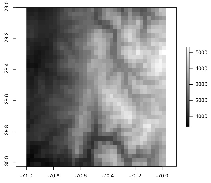
An example of the importance of resolution is illustrated in Figure 1. As resolution decreases, the relief is smoothed and elevation decreases. Weather models at lower resolution cannot discriminate the impact of mountains, such as wind drag, wind channelling, orographic precipitation, etc. and therefore are less reliable than higher resolution models.
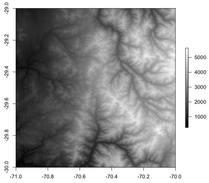 |  |
| a) 30 m | b) 3 km |
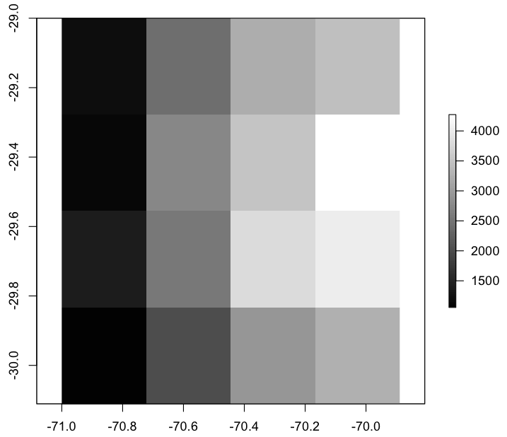 | 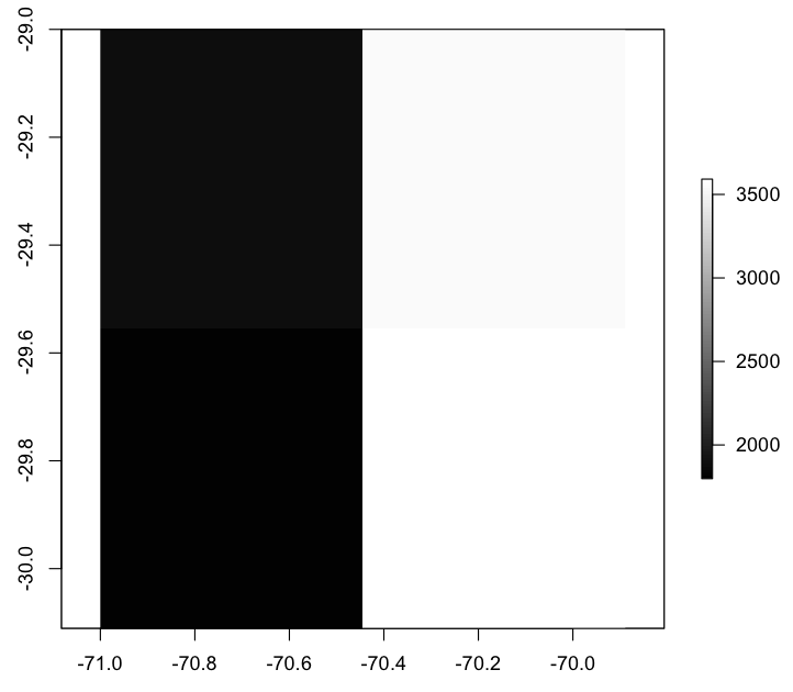 |
| c) 30 km | d) 60 km |
Figure 1 Digital Elevation Model (DEM) of the Arid Andes at different resolution (30 m, 4 km, 30 km and 60 km). Note the highest elevation is in excess of 5000 m at 30 m and 4 km, and only 3500 m at 60 km resolution.
These differences in resolution have a strong impact when modelling wind speed as seen in Figure 2. Note how the WRF, on the right panel, can identify individual valleys and how the wind streams follow the main valleys. This in turn will affect wind velocity and therefore wind energy forecasts, wind potential or the exposure of workers in operations at high altitude.
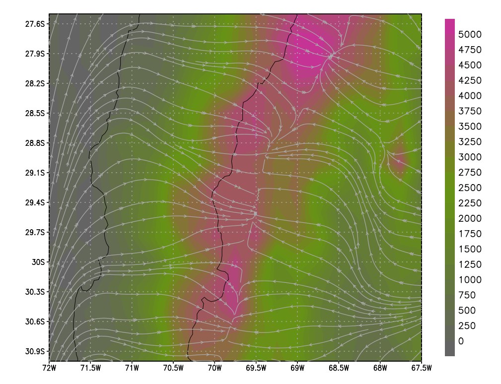 | 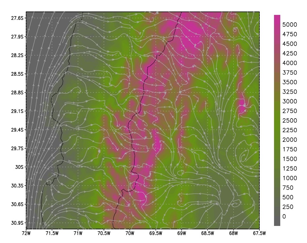 |
| a) GFS 0p25 | b) WRF 3 km |
Figure 2. Surface elevation and wind streams over the Central Arid Andes of Chile And Argentina. On the left panel a GFS simulation at 0.25° resolution, on the right panel a WRF simulation at 4 km resolution.
Wind power density, or power per unit surface area, is calculated as \( P = \frac{1}{2} \rho v^3 \), where \(\rho \) is air density and \(v\) is wind speed. On the charts displayed we have not considered Betz'z Limit, generator efficiency or rotor swept area. Air density is calculated as a function of local pressure, humidity and temperature \( \rho = f(p, RH, T) \) (See for example Brutsaert, 1983 and Jacobson, 1999).
Power curves are plotted from data provided by the manufacturer or published by NREL (National Renewable Energy Laboratory). If data are missing we have used an approximation to the non-linear part of the curve provided Carrillo et al., 2013. If you have more accurate data for your own generators, please let us know and we will include them.
Regonal maps show the relative wind energy production by region. Wind speed index is the average wind speed at 80 m above ground level in all wind generators in the region. Wind power index is an arbitrary index estimated as \( Idx = \sum_{n=1}^{n=ber of sites}(WPD*IP) \), where WPD is wind power density at 80 m and IP is installed power. This index is not a real value of power generation, but an indication of potential production. The actual value can be estimated on demand.
Maps fronm the WRF and GFS model are provided to give an idea of the regional weather, as well as satellite maps in the visible, IR and water vapor bands plus derived precipitation intensity. we also provide a link to MODIS high resolution (250 m) images
Brutsaert, W., 1982: Evaporation into the atmosphere : theory, history, and applications. Kluwer Academic, Dordrecht, 316 pp.
Carrillo, C., A. F. Obando Montaño, J. Cidrás, and E. Díaz-Dorado, 2013: Review of power curve modelling for wind turbines. Renew. Sustain. Energy Rev., 21, 572–581, doi:10.1016/j.rser.2013.01.012. http://www.sciencedirect.com/science/article/pii/S1364032113000439.
Jacobson, M. Z., 1999: Fundamentals of Atmospheric Modeling.Cambridge University Press,.
Some of our related publications
Durand, Y., G. Guyomarc’h, L. Merindol, J. G. Corripio, G. Giraud, E. Brun, and E. Martin, 2003: Ten years of operational numerical simulations of snow and mountain weather conditions and recent developments at Météo-France. Proc. Int. Conf. Alp. Meteorol. (ICAM/MAP Conf. Switzerland, from May 19 to 23, 2003,.
Durand, Y., G. Guyomarc’h, L. Mérindol, and J. G. Corripio, 2004: 2D numerical modelling of surface wind velocity and associated snow drift effects over complex mountainous oragraphy. Ann. Glaciol., 38, 59–70.
Durand, Y., G. Guyomarc’h, L. Mérindol, and J. G. Corripio, 2005: Improvement of a numerical snow drift model and field validation. Cold Reg. Sci. Technol., 43, 93–103.