We’ll have a quick look at some of the functions in the R package insol. Here we will learn to calculate shadows and illumination intensity and to compute insolation on solar panels, windows or complex terrain. There is a basic description of the background processes which involve vector algebra. It helps to understand how it works, but it is not needed for practical applications.
Background
R insol follows the algorithms developed in Corripio (2003), which treat the sun and every grid cell as a vector. A usual terrain representation is a Digital Elevation Model (DEM), that is a matrix of terrain elevation (Z) at given regular spacing in the X (eastings) and Y (northings) direction. Because most modern computer languages are very efficient at dealing with matrices, these solar algorithms are quite fast.
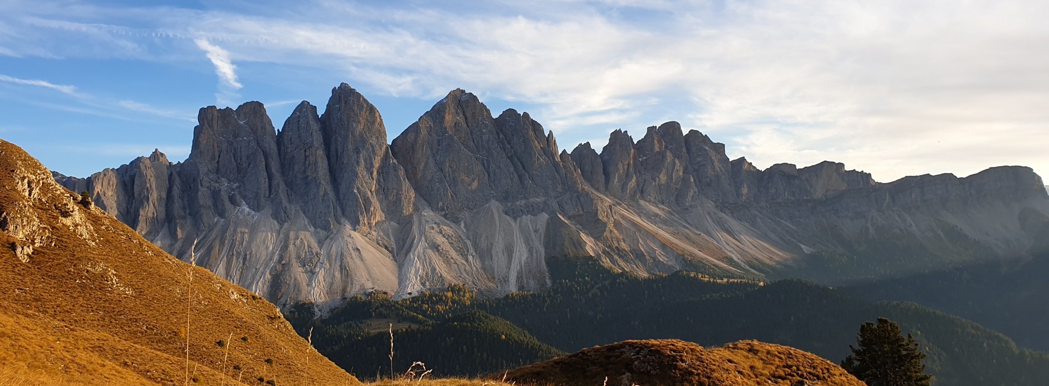
We define the sun vector as a unit vector pointing towards the sun in a reference system fixed on the observer, as in the figure below. Direction of the axes are arbitrary, as long as they are consistent. In this case we chose X as east-west and positive eastwards, Y as north-south and positive southwards, and Z along the Earth radius and positive upwards.
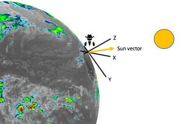
Figure 1.- Representation of the vector defining the position of the sun
The terrain is treated as a matrix of unit vectors perpendicular to every grid cell in the DEM. It is calculated as the cross product  in Figure 2, or rather the average and
  as 4 points are not necessarily on the same plane. Function
 cgrad() in insol makes the computation and returns a 3D Matrix with the same number of rows and columns as the DEM and the 3 layers corresponding to the x, y and z components of the normal vectors. In this way to estimate the illumination intensity we only need to compute the dot product of the sun vector with every vector normal to the grid terrain. The dot product of two unit vectors is equal the cosine of the angle between the vectors, in the same way that illumination intensity is proportional to the cosine of the angle between the sun and the surface. The illumination intensity would be  . Note that
  in Figure 2 is the opposite direction than in Figure 1, but it is shown that way for clarity.
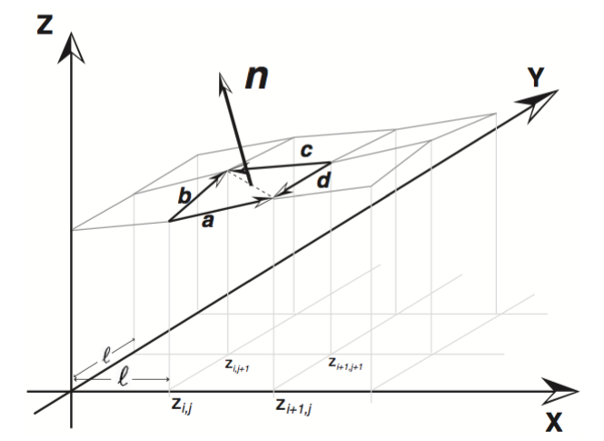
Figure 2.- Terrain representation as a Digital Elevation Model and vector normal to every grid cell.
Relief shading of a geometric shape
These algorithms are ready to use in the R package insol. To produce the cone shadow animation at the beginning of the post requires only a few lines of code. First, let’s create the actual cone:
# let's create a cone
cone = function(x, y){sqrt(x^2+y^2)}
x = y <- seq(-1, 1,length=200)
z = outer(x, y, cone)
# pointing up and removing squared sides
z = max(z)-min(z[,1])-z
z[z<0] = 0
# vertical enhancement and proportional cell size
z = z*300
cellsize = 1
#let's have a look:
persp(x,y,z)
We insert that cone in the middle of a larger DEM to be able to visualise the shadows, then run an example with illumination at 45° elevation, 315° azimuth, as shown in Figure 3. Placing the cone in the middle let us visualise shadows both in the northern and southern hemisphere.
# let's create a cone
cone = function(x, y){sqrt(x^2+y^2)}
x = y <- seq(-1, 1,length=200)
z = outer(x, y, cone)
# pointing up and removing squared sides
z = max(z)-min(z[,1])-z
z[z<0] = 0
# vertical enhancement and proportional cell size
z = z*300
cellsize = 1
#let's have a look:
persp(x,y,z)
Figure 3.- DEM of a cone with illumination at 45° from the North West.
To replicate the initial animation we can simulate the actual illumination from 6 a.m. to 6 p.m for a cone on a flat surface located at the coordinates of Edinburgh Arthur’s Seat on the spring equinox. The following code creates each individual image (145 of them), later they can be processed into a video using ffmpeg, ImageMagick or any other suitable software. For this example we used QuickTime 7 pro.
require(rgl)
lat = 55.943985
lon = -3.161953
xx = 1:1000
yy = 1:1000
open3d(zoom = 0.85, windowRect=c(20,65,755,770))
# create an array of julian dates from 6 a.m. to 6 p.m at 5 minutes interval
jd = JD(seq(ISOdate(2019,3,20,6),ISOdate(2019,3,20,18),by="5 min"))
# set the preferred orientation of the image with the mouse before doing
# the following loop, or use rgl.viewpoint() or userMatrix
i = 1
for (jdt in jd){
    print(paste("Timestep ",i,"of",length(jd),jdt))
    sv = sunvector(jdt, lat, lon, 0)
    hsh = grd[,,1]*sv[1]+grd[,,2]*sv[2]+grd[,,3]*sv[3]
    hsh = (hsh+abs(hsh))/2
    sh = doshade(dem,sv,cellsize)
    hshsh = hsh*sh
    hshsh=(t(hshsh[nrow(sh):1,]))
    pngname = paste('coneshadow',i,'.png',sep='')
    clear3d()
    terrain3d(xx,yy,dem,col=grey(hshsh),lit=FALSE)
    rgl.snapshot(pngname)
    i=i+1
}
Relief shading of complex topography
To apply illumination and shading to an actual DEM of complex topography, we can use the example provided for the Ordesa National Park in the Pyrenees. It is recommended to use the package raster, to get the actual geographical extent and latitude to longitude ratio. Insol requires a regular squared grid cell, that means that UTM projection is OK, but geographical latitude, longitude is not, as the actual interval in longitudes varies wth the latitude. First let’s download the DEM:
library(raster)
demfile = tempfile()
download.file("http://www.meteoexploration.com/R/insol/data/dempyrenees.tif",demfile)
dem = raster(demfile)
grd = cgrad(dem)
lat = 42.647
lon = -0.017
# sunvector at 9:15 local time
jd = JD(ISOdatetime(2019,3,20,10,55,40))
sv = sunvector(jdt, lat, lon, 0)
hsh = grd[,,1]*sv[1]+grd[,,2]*sv[2]+grd[,,3]*sv[3]
## remove negative incidence angles (self shading)
hsh = (hsh+abs(hsh))/2
hsh = raster(hsh,crs=projection(dem))
extent(hsh) = extent(dem)
sh = doshade(dem,sv)
hshsh = hsh*sh
plot(hshsh,col=grey(1:100/100),legend=FALSE)
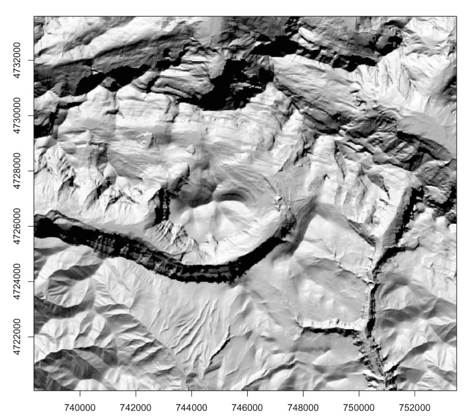
Figure 4.- Simulated insolation and shading on the Ordesa National Park in the Pyrenees in spring.
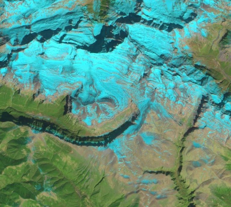
Figure 5.- Sentinel-2 image cropped to the same region as in Figure 4.
The Sentinel image is a false colour representation where snow appears light blue. The image is taken near midday and illumination is from the South. This type of illumination is difficult to interpret and can cause relief inversion, with protruding valleys and sinking peaks, thats why a common illumination in maps is from the northwest (see more about relief inversion here). If we rotate the images the relief is appreciated correctly and more easily, as in Figure 6.
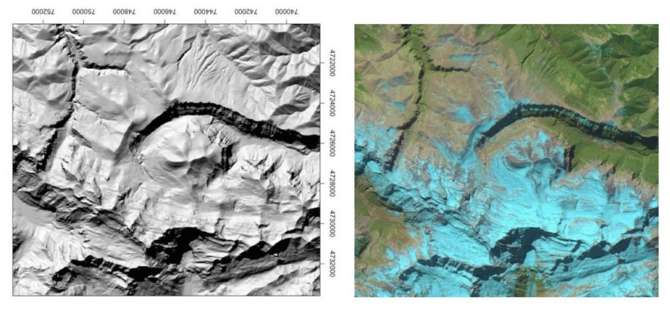
Figure 6.- As Figure 5 and 6 rotated 180°
Insolation on solar panels or windows
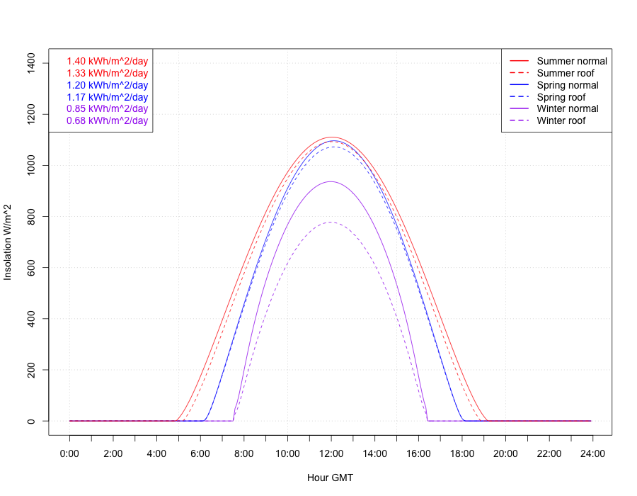
Figure 7.- Insolation on solar panels at a mountain hut in the Pyrenees.
The same approach can be used to estimate insolation on a window, for energy efficiency calculations in buildings. A vertical window facing southeast would be defined by the vectorwv=normalvector(90,135). The rest of the calculations are the same, although it should include shading from nearby buildings or the roof. R insol and climatic data have been used to produce high resolution the solar radiation maps in this link.
Please check the manual, references and help in the code, either at our pages or the CRAN repository, for a more detailed discussion. The main algorithms are described in the paper below. We hope you can find the package useful.
References
Corripio, J. G.: 2003, Vectorial algebra algorithms for calculating terrain parameters from DEMs and the position of the sun for solar radiation modelling in mountainous terrain, International Journal of Geographical Information Science 17(1), 1–23. PDF
R project Manuals and Documentation